
Overview
The United States has seen an unsustainable increase in the cost of health care in recent decades. Many Americans are now afraid of seeking treatment, and those that do are often left with unexpectedly high medical bills that become a major financial burden.
Our goal for this project is to offer quick and accurate predictions of health insurance costs for an individual without reliance on his or her previous medical expenses. We hope that these predictions will help individuals choose appropriate health insurance plans and make more informed financial decisions.
To accomplish this task, we trained multiple regression models with the dataset below and evaluated their performance by comparing each R2 Score and MSE. We repeated this process for both high costs only and low costs only in an attempt to make better predictions for individuals who are highly likely to belong in one of these categories. Through our exploratory data analysis and unsupervised learning, we identified the factors that would make an individual more likely to experience high costs, and a dollar amount to split the dataset on to distinguish between high and low costs.
Dataset
Our dataset is from Kaggle and contains a mix of numerical and categorical data. The features include:
- Age: integer
- Sex: male or female
- BMI: decimal
- Number of children: integer
- Smoker: yes or no
- Region (US): southeast, southwest, northeast, or northwest
- Charges: decimal (ground truth)
Data Cleaning
Before working with our dataset, we wanted to ensure that it was thoroughly cleaned and usable so that it would not affect the results of our unsupervised or supervised learning. The steps we took to clean our data were:
- Removing rows with missing values
- Removing duplicate rows
- Removing rows with bad values (ex: charges less than zero)
In addition to these steps, we also performed a one-hot encoding on the data, converting features such as smoker from “yes” and “no” to 1 and 0. One of our features, region, was encoded in two different ways for use in different parts of our project. First, our four regions were encoded as 0, 1, 2, and 3 for use in data exploration. However, this encoding would become a problem in our unsupervised learning, since when measuring euclidean distance, the regions encoded as 0 and 3 would be seen as further apart than 0 and 1, even though there is no true meaning for this larger difference between the regions. Therefore, our second encoding had region split into four separate features, one for each region, so that no pair of regions would be seen as further apart than another.
Data Exploration
To start our data exploration, we created a heat map to analyze the correlation between the different features and the target. From this heat map we noticed that smoking was highly correlated with charges, and both bmi and age were moderately correlated with charges. Since smoking, bmi, and age were the features most correlated with charges, we decided to look at these relationships more closely.

Smoking appears to have a significant impact on charges. We found that smokers tend to have charges from about $20,000 - $40,000, while non-smokers have much lower charges from about $5000 - $10000.

When analyzing BMI and charges, it appears that upon reaching a BMI greater than 30, the population separates significantly. After this point it appears that some members of the population have charges that are double or triple that of others. After applying a hue to the plot indicating smoking status, we can see that charges for smokers increase linearly with BMI, while non-smoker charges remain fairly constant as BMI increases. This again shows the significant impact of smoking, which is worsened by a higher BMI.

Since poor BMI seems to lead to higher charges, we decided to further analyze this trend. Any member of the population with a BMI greater than 25 was labeled overweight, and others not overweight. After comparing the two groups, it appears that most members of each group have charges around $8000. However, it is clear that those who are overweight are more likely to suffer high charges compared to those who are not.

The last relationship we chose to look at was between age and charges. As expected, increased age generally leads to increased charges, but like bmi, there appears to be distinct groups in the population with vastly different charges. When applying the smoker hue once again, it can be seen that charges for both smokers and non-smokers increase with age, but smokers have much higher charges overall.

The results of this data exploration lead us to believe that smoking is by far the most important feature in determing an individual’s risk for high insurance costs, with age and BMI still playing a modest role. Since smoking has such strong influence, we believe the best split between high and low cost should be defined by the separation between charges for smokers and non-smokers. We will confirm and expand upon this claim in our unsupervised results section.
Unsupervised Learning
Principal Component Analysis
Despite already having a low number of features, we decided to use PCA to see if we could further reduce the dimensionality. After performing PCA on our scaled features, we plotted the principal components against cumulative explained variance and found that we would need 8 out of 9 of these components to explain 99% of the total variance. Since this reduction from our existing dataset is very minor, we believe that it is not valuable to reduce the dimensionality.

Clustering
KMeans
The first clustering method we utilized was KMeans. Since this method relies on euclidean distance to create clusters, we scaled all features to the range (0, 1) so that clustering was not dominated by our larger features. After running KMeans on our scaled features, it appeared difficult to find meaningful clusters. However, by using the elbow method and silhouette coefficients, we decided that we would be able to gain valuable information from 15 clusters.


KPrototype
Another method that we attempted to use was KPrototype clustering. Since we have a mix of numerical and categorical data, many traditional clustering algorithms are difficult to apply to our data. In KPrototype clustering, similiarity is determined by comparing numerical and categorical data differently. After specifying which features are categorical, the algorithm will cluster the data using, for example, euclidean distance for numerical features and hamming distance for categorical features. By using this method we were able to achieve slighly improved distortion values, but ultimately we found our KMeans clustering to be more useful for understanding our data and accomplishing our task.

Unsupervised Results
As stated previously, even though it was difficult to find meaningful clusters, we were able to gain valuable information from using KMeans with 15 clusters that confirmed our earlier data exploration findings. When observing the average and standard deviation of the charges in each cluster, it is clear that some clusters primarily have much lower charges than others. To investigate this phenomenon, we looked at the average and standard deviation of each feature for each cluster. Only one feature offered a clear and meaningful explanation for the difference of charges between clusters: smoking. Every cluster that had signficantly higher average charges consisted of only smokers. This evidence confirms the earlier claim made in the data exploration section that smoking is by far the most important feature in determing an individual’s risk for high insurance costs. These results coupled with our earlier findings from data exploration lead us to believe that $15000 is the optimal split between high and low cost insurance, as this represents a split between the charges for smokers and non-smokers.


Supervised Learning
To make the best possible predictions, we compared the performance of four different regression models on combined, high, and low cost data individually. By also training each of our models with high and low cost data only, we hoped to achieve more accurate predictions for individuals highly likely to have low or high costs, which we now know is significantly influenced by smoking and potentially a higher BMI.
We used our unsupervised results to determine the threshold to split high cost versus low cost for our supervised learning. After creating our high and low cost datasets based on our $15000 threshold, we created a training and testing set for each, as well as for the combined dataset. Each training set consisted of 80% of the data in a set, while each testing set consisted of the remaining 20%. All data in both training and testing sets was scaled so that evaluation metrics were interpretable, and the performance of scaled sets was compared against unscaled sets to ensure that performance was unaffected.
Linear Regression
Linear Regression is among the most common approaches we have seen others use to predict insurance costs. Since this method is so common, we decided to use it as a starting point to compare to our chosen models. This method did not require any hyperparameter tuning and was not one of our primary methods.


Random Forest
The first of our chosen models we decided to evaluate was Random Forest since this method has been shown to provide accurate results in wide variety of similar problems. As an implementation, we used Scikit-learn’s RandomForestRegressor. Using bootstrap aggregating allowed us to achieve better results from this model, independent of other parameters, so we chose to keep this constant as we searched for our other optimal parameters with RandomizedSearch. These parameters included the number of trees, column ratio for each tree, max tree depth, min samples for a split, and min samples to be a leaf.
The search space for RandomizedSearch was set as follows after manual tuning and run for 300 iterations:
- Number of trees: 100 - 200 (inc of 1)
- Column ratio for each tree: 0.5 - 0.9 (inc of 0.1) and auto
- Auto is equivalent to using all of the columns
- Max tree depth: 2 - 10 (inc of 1)
- Min samples for a split: 2 - 10 (inc of 1)
- Min samples to be a leaf: 1 - 10 (inc of 1)
All Cost Evaluation

High Cost Evaluation

Low Cost Evaluation


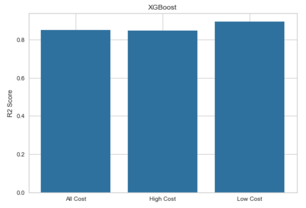
XGBoost
The next model we chose to evaluate was XGBoost. After conducting our research, we learned that XGBoost has been able to make accurate predictions for low cost insurance in the past, so we chose it to try to improve our own low cost predictions. As an implementation, we used XGBRegressor from the xgboost library. For the learning objective, we found that reg:squarederror produced the best results, so we decided to keep this objective constant while tuning other parameters with RandomizedSearch. These parameters included the number of gradient boosted trees, max tree depth, learning rate, gamma, subsample ratio for each tree, and column ratio for each tree.
The search space for RandomizedSearch was set as follows after manual tuning and run for 300 iterations:
- Number of gradient boosted trees: 100 - 200 (inc of 1)
- Max tree depth: 2 - 10 (inc of 1)
- Learning rate: 0.01 - 0.2 (inc of 0.01)
- Gamma: 0.01 - 0.1 (inc of 0.01)
- Subsample ratio for each tree: 0.5 - 1 (inc of 0.1)
- Column ratio for each tree: 0.5 - 1 (inc of 0.1)
All Cost Evaluation

High Cost Evaluation

Low Cost Evaluation


Artificial Neural Network
The last model we chose to evaluate was ANN. After conducting our research, we learned that ANN has been able to make accurate predictions for high cost insurance in the past, so we chose it to try to improve our own high cost predictions. As an implementation, we used Scikit-learn’s MLPRegressor. Since our dataset is not very large, we used the lbfgs solver for weight optimization, as this solver is known to help smaller datasets converge faster and perform better. We also chose to use one hidden layer since we discovered that only one was necessary for most other problems of similar scale and complexity. To optimize the remaining parameters, we again made use of RandomizedSearch. These parameters included the maximum number of iterations, size of our hidden layer, activation function, and alpha value.
The search space for RandomizedSearch was set as follows after manual tuning and run for 300 iterations:
- Maximum iterations: 500 - 1000 (inc of 100)
- Values in this range allowed the model to converge most of the time
- Size of hidden layer: 2 - 7 (inc of 1)
- Size of the hidden layer should be between the size of the input and output layer
- Activation function: tanh or relu
- Alpha: 0.0001 - 0.0009 (inc of 0.0001)
All Cost Evaluation

High Cost Evaluation

Low Cost Evaluation


Supervised Results
After training and evaluating our models with different combinations of parameters, we compared the R2 scores and MSE values of each to determine which offered the best predictions for all, high, and low costs. A common problem we found was a decrease in performance on high cost data only. This proved to be significant for linear regression and ANN, and noticeable for Random Forest and XGBoost. We believe that this is caused by the low number of observations in the high cost training set, so there was little we could do to address this issue. On the other hand, our best results were from low cost data only, which demonstrates the value of our decision to split. Below is a summary of our supervised metric evaluation.
R2 Score Results

MSE Results

All Costs
For our all costs dataset, we found that ANN had the best performance with XGBoost and Random Forest following closely behind. This was a surprising discovery, since we expected ANN to have the best results for high cost data. However, ANN ended up performing significantly worse on high cost data, and as mentioned previously, we believe that this is because of the lack of observations in the set. With more observations in the training set, we believe that ANN would perform the best on the high cost set, but we are glad this method still proved to be useful. We found that 500 iterations, 4 nodes in our hidden layer, relu activation function, lbfgs solver, and an alpha value of 0.0009 led to the best performance for this model on all costs. The predictive performance of this model is shown below.

High Costs
For our high costs dataset, we found that XGBoost had the best performance with Random Forest following closely behind. We found that a squared error learning objective, 166 trees, max depth of 3, column ratio for each tree of 0.9, subsample ratio for each tree of 1, learning rate of 0.06, and gamma value of 0.1 led to the best performance for this model on high costs. The predictive performance of this model is shown below.

Low Costs
For our low costs dataset, we found that XGBoost again had the best performance with ANN following extremely closely behind. We found that a squared error learning objective, 195 trees, max depth of 2, column ratio for each tree of 0.6, subsample ratio for each tree of 1, learning rate of 0.07, and gamma value of 0.01 led to the best performance for this model on low costs. The predictive performance of this model is shown below.

Conclusion
Our goal for this project was to provide accurate predictions of health insurance costs for an individual so that he or she would be able to choose appropriate health insurance plans and make more informed financial decisions. By conducting an exploratory data analysis and clustering our features, we found that smokers tend to have much higher charges along with some influence from increased BMI, and identified a value of $15000 to split our dataset into high and low cost data. By splitting our dataset, we hoped to provide even more accurate predictions for those highly likely to fall within one of the two categories of insurance costs. After training and evaluating the performance of our supervised models on all cost data, we were able to achieve a highest R2 score of 0.857 and lowest MSE of 0.164. By utilizing our low cost dataset, we were able to improve predictions for those likely to have low costs, with a highest R2 score of 0.894 and lowest MSE of 0.113. We were not as happy with our results for high cost data only, and we believe that lack of training data in this set was the cause for lower results. In future work, we would want to gather more training data to see if we could also provide better predictions for those likely to have higher insurance costs. Overall we are pleased with our predictions, and hope that others continue to work on this rapidly growing issue.
References
Morid, M., Kawamoto, K., Ault, T., Dorius, J., & Abdelrahman, S. (2018, April 16). Supervised Learning Methods for Predicting Healthcare Costs: Systematic Literature Review and Empirical Evaluation.
Jödicke, A. M., Zellweger, U., Tomka, I. T., Neuer, T., Curkovic, I., Roos, M., . . . Egbring, M. (2019). Prediction of health care expenditure increase: How does pharmacotherapy contribute? BMC Health Services Research, 19(1). doi:10.1186/s12913-019-4616-x
Bertsimas, D., Bjarnadóttir, M. V., Kane, M. A., Kryder, J. C., Pandey, R., Vempala, S., & Wang, G. (2008). Algorithmic Prediction of Health-Care Costs. Operations Research, 56(6), 1382-1392. doi:10.1287/opre.1080.0619